Growth-rate measurement with type Ia supernovae within the ZTF photometric survey
Bastien Carreres
Image credits: ZTF.Caltech
Outline
Introduction:
The $\Lambda$CDM standard model
Modified gravity
Growth rate of structure
What is the growth rate of structure?
How to measure it?
Type Ia supernovae
What are they?
The Zwicky Transient Facility
The growth-rate analysis pipeline
Simulation
Analysis
Results
The sample bias
ZTF 6-years forecast
How to improve the measurement?
Other projects
Systematic effect on $H_0$ due to velocities
What's next?
Conclusion
The standard cosmological model: General Relativity + $\Lambda$CDM
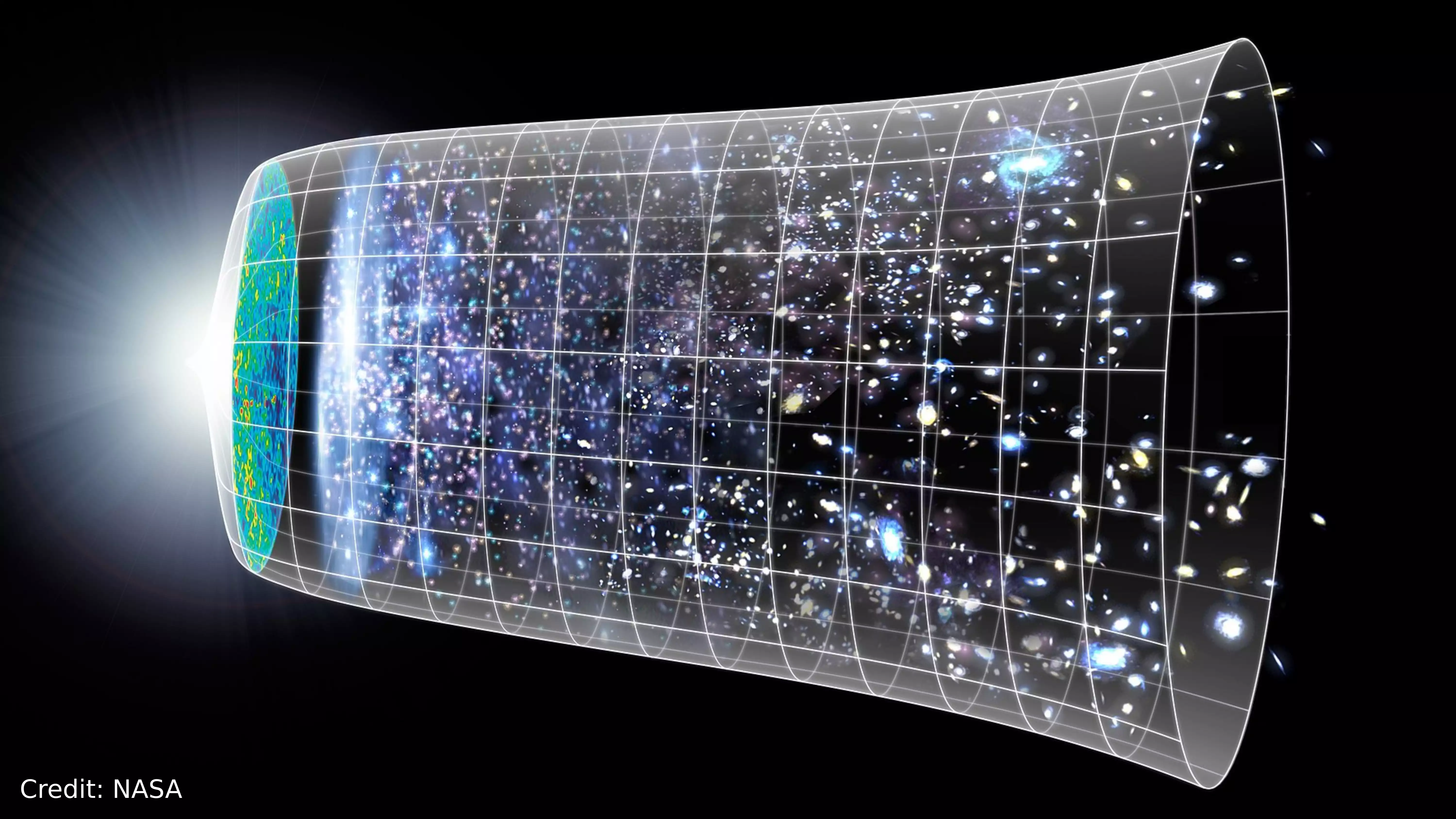
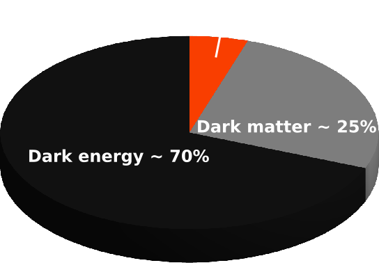
What is dark energy? Is there an alternative to $\Lambda$?
Modified gravity
Many models propose to explain accelerated expansion using new laws for gravity:
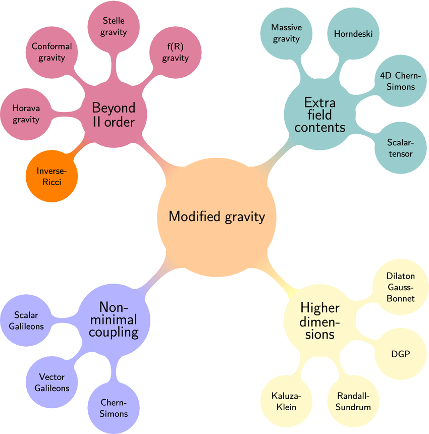
Changing gravity will affect structures formation
Image credits: arXiv:2204.06533
Outline
Introduction:
The $\Lambda$CDM standard model
Alternatives to $\Lambda$
Growth rate of structure
What is the growth rate of structures?
How to measure it?
Type Ia supernovae
What are they?
The Zwicky Transient Facility
The growth-rate analysis pipeline
Simulation
Analysis
Results
The sample bias
ZTF 6-years forecast
How to improve the measurement?
Other works
Systematic effect on $H_0$ due to velocities
What's next?
Conclusion
\(f\sigma_8\) as a probe for general relativity
Structure evolution:
Dark energy vs Gravity
Density contrast: $\delta(\mathbf{x}) = \frac{\rho(\mathbf{x})}{\bar{\rho}} - 1$
$\sigma_8$:
RMS of fluctuation over sphere of
8 Mpc.$h^{-1}$ radius
$\delta(\mathbf{x}) = \sigma_8 \tilde{\delta}(\mathbf{x})$
Velocities are linked to density through the continuity equation:
$\nabla.v(\mathbf{x}) \propto f\sigma_8 \tilde{\delta}(\mathbf{x})$
where $f \equiv$ growth rate
General Relativity + $\Lambda$CDM:
$f \simeq \Omega_m^\gamma$ with $\gamma \simeq 0.55$

Image credits: Illustris TNG
How to measure $f\sigma_8$ ?
Velocities as probes of $f\sigma_8$:
$\nabla.v \propto f\sigma_8$
Doppler effect on redshift:
$1 + z_\mathrm{obs} = \left(1 + z_\mathrm{cos}\right)\left(1 + z_p\right)$
$z_p \simeq \frac{v_p}{c}$, $v_p$ is the line-of-sight velocity
$v_p \sim 300 \ \mathrm{km}.\mathrm{s}^{-1}$ and $z_p \sim 0.001$
Direct velocity tracers
Data: redshifts + distances
Galaxies Tully-Fisher and Fundamental Plane: $\sigma_D/D \sim 20\%$
Type Ia supernovae: $\sigma_D/D \sim 7 \%$


Galaxies: Tully-Fisher & Fundamental plane relation
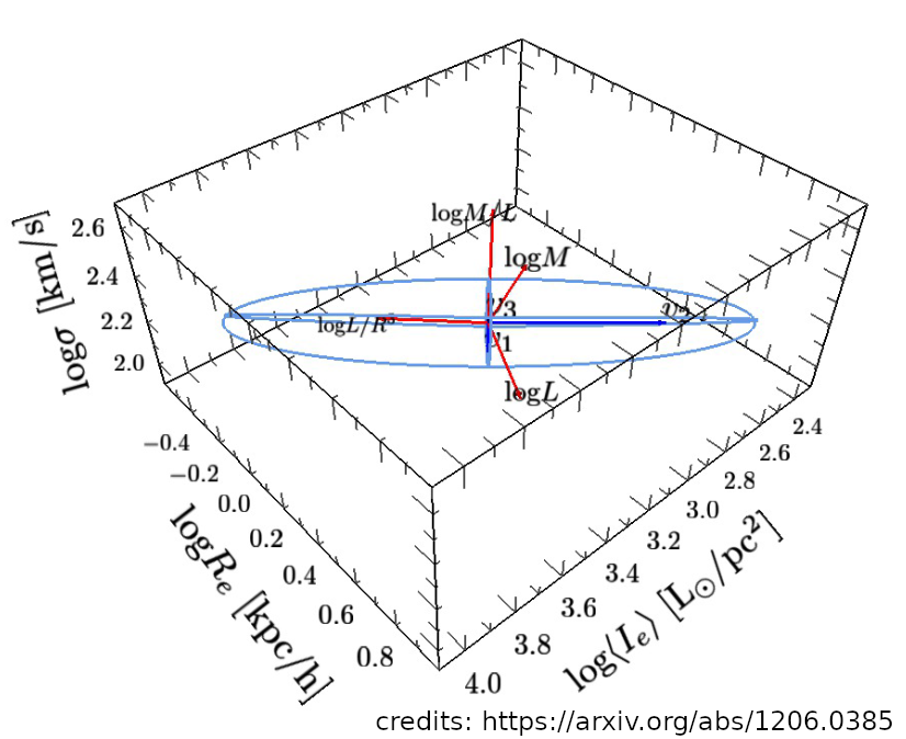
Image credits: Illustris TNG
Outline
Introduction:
The $\Lambda$CDM standard model
Alternatives to $\Lambda$
Growth rate of structure
What is the growth rate of structures?
How to measure it?
Type Ia supernovae
SNe Ia for cosmology
The Zwicky Transient Facility
The growth-rate analysis pipeline
Simulation
Analysis
Results
The sample bias
ZTF 6-years forecast
How to improve the measurement?
Other works
Systematic effect on $H_0$ due to velocities
What's next?
Conclusion
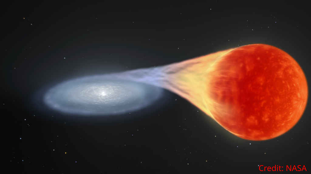
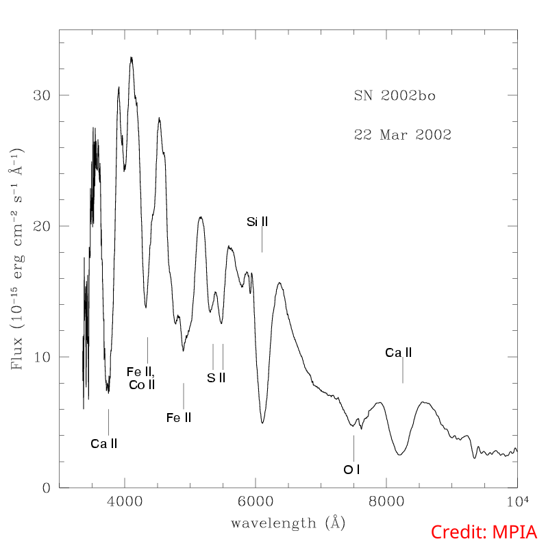
Type Ia supernovae (SNe Ia): powerful probes for cosmology
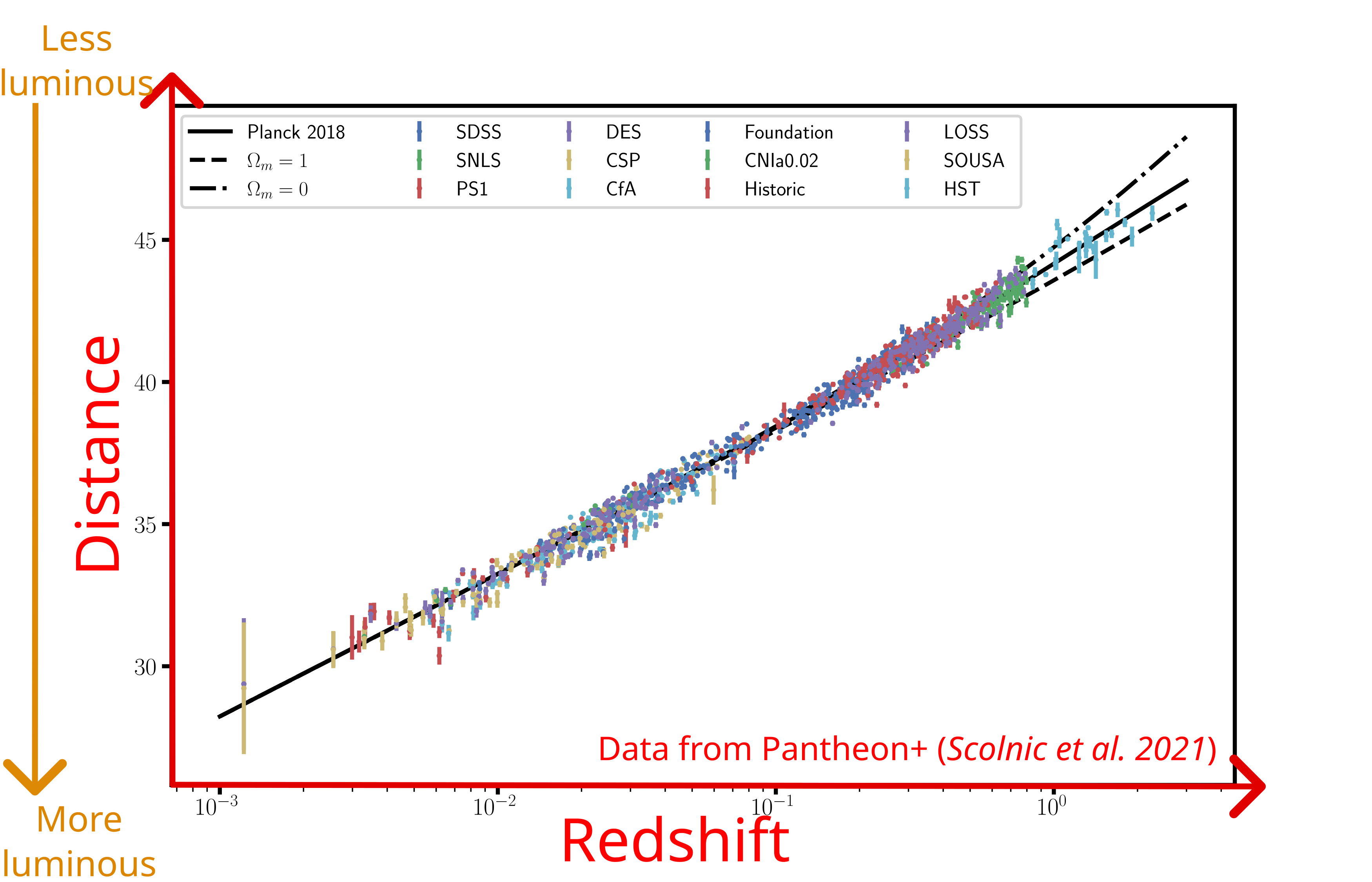
Distance modulus: $\mu = m_B - M_B \propto 5\log(d_L)$
SNe Ia: a few words about standardization
SNe Ia are not perfectly standard !!!
Correlation of peak magnitude with stretch, color and host galaxies exists
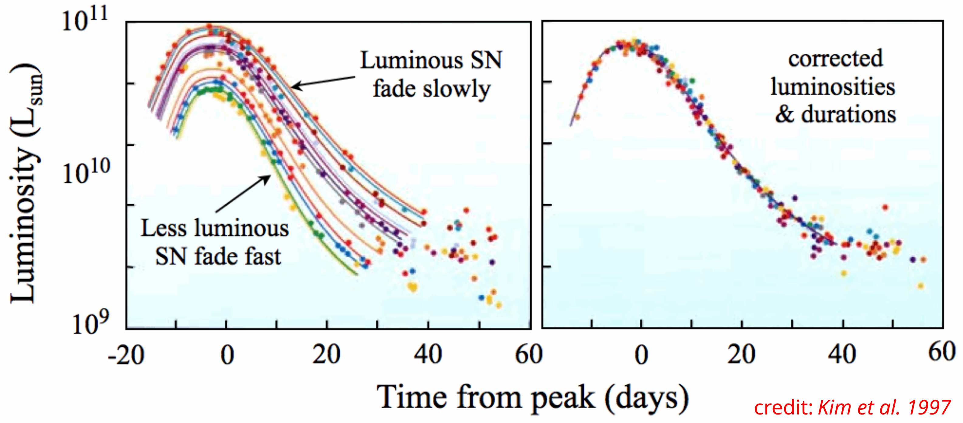
Tripp relation: $m_B^\mathrm{std} = m_B + \alpha x_1 - \beta c$
After standardization $\sigma_M \sim 0.12$
How to get $m_B$, $x_1$ and $c$?
Collect data
Adjust lightcurve with SALT2 (SED model for SNe Ia)
The Zwicky Transient Facility survey
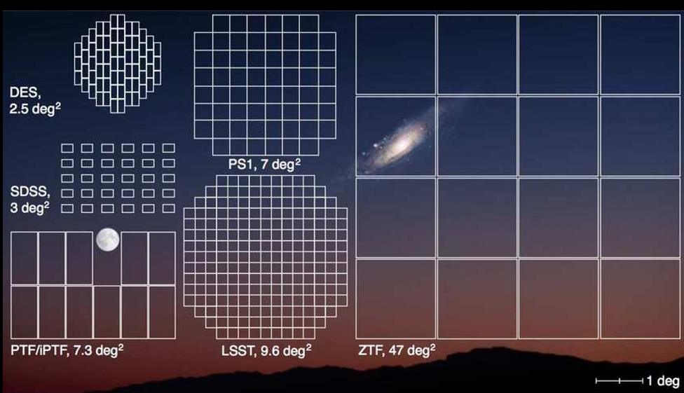
The ZTF survey:
Photometric telescope observing 3/4 of the sky every $\sim 2$ nights in 3 bands
Spectroscopic telescope measuring transient spectra
$\sim 8000$ classified supernovae
More than 3000 SNe Ia at low redshift $z < 0.1$
Image credits: ZTF.Caltech
Outline
Introduction:
The $\Lambda$CDM standard model
Alternatives to $\Lambda$
Growth rate of structure
What is the growth rate of structure?
How to measure it?
Type Ia supernovae
SNe Ia for cosmology
The Zwicky Transient Facility
The growth-rate analysis pipeline
Simulation
Analysis
Results
The sample bias
ZTF 6-years forecast
How to improve the measurement?
Other works
Systematic effect on $H_0$ due to velocities
What's next?
Conclusion
$f\sigma_8$ with SNe Ia peculiar velocities: the simulation and analysis pipeline
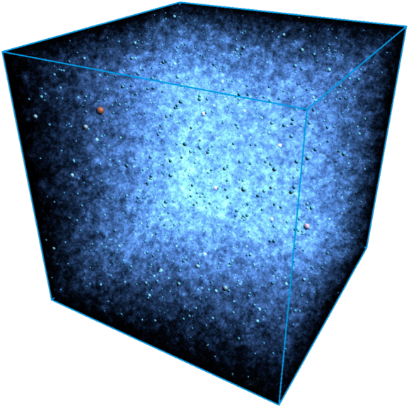
Simulation: the N-Body simulation
OuterRim (Heitmann et al. 2019)
WMAP cosmology, $f\sigma_8 = 0.382$
(3 Gpc.$h^{-1}$)$^3$ box of dark matter halos at $z=0$
$\Rightarrow$ 27 ZTF realisations up to $z\sim 0.17$
Simulation: SN Ia model
$1 + {\color{#96F1FD}z_\mathrm{obs}} = (1 + {\color{#96F1FD}z_\mathrm{cos}}) (1 + {\color{#96F1FD}z_\mathrm{p}})$
$m_{B,i} = {\color{#E78A0D}M_B} - {\color{#E78A0D}\alpha x_{1, i}} + {\color{#E78A0D}\beta c_i }+ {\color{#E78A0D}\sigma_{\mathrm{int}, i}} + \mu({\color{#96F1FD}z_{\mathrm{cos},i}}) + 10\log(1 + {\color{#96F1FD}z_{p,i}})$
Simulation: survey parameters
I have worked in ZTF simulation working group to construct ZTF simulation input files

Simulation: $\texttt{SNSim}$ and lightcurves
Noise is computed as
$\sigma_F = \sqrt{F + \sigma_\mathrm{sky}^2 + \sigma_\mathrm{ZP}^2}$
Simulation: applying spectroscopic identification selection function
Detection: 2 points with SNR $>$ 5
Spectroscopic efficiency from Perley et al. 2019
$\langle N_\mathrm{SN} \rangle\sim 4300$

$f\sigma_8$ with SNe Ia peculiar velocities: the simulation and analysis pipeline
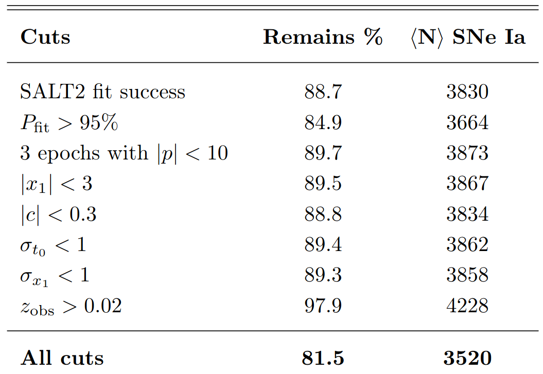
Analysis: lightcurves fit and cosmological cut
After SALT2 fit, we apply quality cuts:
Analysis: velocities from Hubble diagram residuals
Standard candles
Standard candles + velocities
Standard candles + velocities + noise
The velocity estimator:
$$\hat{v} = -\frac{\ln(10)c}{5}\left(\frac{(1+z)c}{H(z)r(z)} - 1\right)^{-1}\Delta\mu$$
The velocity estimator error:
$$\sigma_\hat{v} = -\frac{\ln(10)c}{5}\left(\frac{(1+z)c}{H(z)r(z)} - 1\right)^{-1}\sigma_\mu$$


Analysis: the Maximum-Likelihood method
Method used with galaxy data in Abate et al. 2010, Johnson et al. 2014 and Howlett et al. 2017

The correlation function depends on the Power Spectrum
$\langle v(\mathbf{x}_i)v(\mathbf{x}_j)\rangle \propto (f\sigma_8)^2 \int dk \tilde{P}(k) W^{(v)}(k; \mathbf{x}_i, \mathbf{x}_j)$
It gives us a $f\sigma_8$ dependent model for our covariance matrix!
$C_{ij}^{vv}(f\sigma_8) = \langle v(\mathbf{x}_i)v(\mathbf{x}_j)\rangle$
- One based on N-body simulaton fit from Bel et al. 2019
- One based on PT beyond order one from Taruya et al. 2012
Effect of redshift space distorsions taken into account with damping function $D_u(\sigma_u)$ (Koda et al. 2014)

Analysis: the Maximum-Likelihood method
Free parameters of the likelihood:
${\color{yellow} \mathbf{p} = \left\{f\sigma_8, \sigma_u, \sigma_v \right\}}$, $\sigma_u \equiv$ RSD, $\sigma_v\equiv$ non-linearities
The likelihood:
$\mathcal{L}({\color{yellow}\mathbf{p}}) \propto |C({\color{yellow}\mathbf{p}})|^{-\frac{1}{2}} \times\exp\left[-\frac{1}{2}\mathbf{v}^TC({\color{yellow}\mathbf{p}})^{-1}\mathbf{v}\right]$The covariance:
$C_{ij}({\color{yellow}\mathbf{p}}) = C^{vv}_{ij}({\color{yellow}f\sigma_8}, {\color{yellow}\sigma_u}) + {\color{yellow}\sigma_v}^2 \delta^K_{ij} + \sigma_\hat{v}^2 \delta^K_{ij}$$C^{vv}_{ij}({\color{yellow}f\sigma_8}, {\color{yellow}\sigma_u}) = \langle v(\mathbf{x}_i)v(\mathbf{x}_j)\rangle \propto ({\color{yellow}f\sigma_8})^2 \int dk P(k) W(k) D_u^2(k; {\color{yellow}\sigma_u}) $
Outline
Introduction:
The $\Lambda$CDM standard model
Alternatives to $\Lambda$
Growth rate of structure
What is the growth rate of structures?
How to measure it?
Type Ia supernovae
SNe Ia for cosmology
The Zwicky Transient Facility
The growth-rate analysis pipeline
Simulation
Analysis
Results
The sample bias
ZTF 6-years forecast
How to improve the measurement?
Other works
Systematic effect on $H_0$ due to velocities
What's next?
Conclusion
Results: the selection bias (Carreres et al. 2023)
Bias on HD residuals

Bias on velocity estimates

$$\hat{v} = -\frac{\ln(10)c}{5}\left(\frac{(1+z)c}{H(z)r(z)} - 1\right)^{-1}\Delta\mu$$

Only the estimated velocities are biased !!!
Bias on $f\sigma_8$

Results: forecast for a ZTF 6-years complete sample (Carreres et al. 2023)
$z \lt 0.06 \Rightarrow \langle N_\mathrm{SN} \rangle \simeq 1600 \sim$ half of the sample
Analysis: joint fit
Free parameters:
Growth-rate related parameters: ${\color{yellow} \mathbf{p} = \left\{f\sigma_8, \sigma_u, \sigma_v \right\}}$SNe Ia Hubble diagram parameters: ${\color{orange} \mathbf{p}_\mathrm{HD} = \left\{\alpha, \beta, M_B, \sigma_M \right\}}$
Data vector
HD residuals: $\Delta \mu({\color{orange} \mathbf{p}_\mathrm{HD}}) = m_B + {\color{orange} \alpha} x_1 - {\color{orange} \beta} c - {\color{orange} M_0} - \mu_\mathrm{model}(z)$$\hat{v} \rightarrow \hat{v}({\color{orange} \mathbf{p}_\mathrm{HD}})= -\frac{\ln(10)c}{5}\left(\frac{(1+z)c}{H(z)r(z)} - 1\right)^{-1}\Delta\mu({\color{orange} \mathbf{p}_\mathrm{HD}})$
Covariance
$\sigma_\hat{v} \rightarrow \sigma_\hat{v}({\color{orange} \mathbf{p}_\mathrm{HD}})= \frac{\ln(10)c}{5}\left(\frac{(1+z)c}{H(z)r(z)} - 1\right)^{-1}\sigma_\mu({\color{orange} \mathbf{p}_\mathrm{HD}})$
Results: forecast for a ZTF 6-years complete sample (Carreres et al. 2023)
$\langle N_\mathrm{SN} \rangle \simeq 1600 \sim$ half of the sample
Results: comparison with existing measurements (Carreres et al. 2023)

With ~1600 SNe Ia, ZTF is at the same precision level as existing measurements with several thousands of galaxies
Results: could a bias correction improve the constraint? (Carreres et al. 2023)
Simulate a perfect correction of the bias: $v_{\mathrm{debias}, i} \sim \mathcal{N}(v_\mathrm{true}, \sigma_{\hat{v}, i})$


How to improve the measurement?
-
Bias correction of the velocity estimates ?
Does not improve strongly the constraint on $f\sigma_8$
Use photo-typing to increase the redshift limit
-
Velocity $\times$ density measurements (e.g. ZTF + DESI)
Future surveys

Forecast credits: DESI arxiv:1611.00036, LSST arxiv:1708.08236, EUCLID arXiv:1606.00180
Outline
Introduction:
The $\Lambda$CDM standard model
Alternatives to $\Lambda$
Growth rate of structure
What is the growth rate of structures?
How to measure it?
Type Ia supernovae
SNe Ia for cosmology
The Zwicky Transient Facility
The growth-rate analysis pipeline
Simulation
Analysis
Results
The sample bias
ZTF 6-years forecast
How to improve the measurement?
Other works
Systematic effect on $H_0$ due to velocities
What's next?
Conclusion
Systematic effect on $H_0$ due to velocities (paper in prep)
Hubble Diagram fit
$\Delta\mu = m_B + \alpha x_1 - \beta c - M_0 - \mu_\mathrm{model}(z)$
where $M_0$ is degenerate with $H_0$
Velocity error term:
$\sigma_{\mu-z} = \frac{5}{\ln 10} \frac{\sigma_v}{z}$
with $c\sigma_v \simeq 250$ km/s
We use our 27 mocks from $\texttt{SNSim}$ that contain correlated velocities to evaluate velocities effect in Hubble diagram fit
Systematic effect on $H_0$ due to velocities (paper in prep)
Velocities not taken into account

Diagonal term for velocity errors

Full covariance matrix for velocities

Preliminary results: using full covariance matrix multiplies by ~4 the error on $M_0$ on simulations. First test on ZTF DR2 data gives an error multiplied by ~2.
What's next?
- Improve the simulation:
- Evaluate the photometric sample:
- Generalisation to velocity-density covariance + improvements of model computation:
- Application of the $f\sigma_8$ analysis to ZTF data
Include more realistic noise, correlation with host properties, color-dependant scattering
Work started with D. Rosselli in a Vera Rubin/DESC project
Work started with C. Ravoux: development of the $\texttt{flip}$ public package
Conclusion
- I developed a simulation of supernovae observations including realistic velocities from N-body simulations
- I used real observation conditions to generate ZTF survey realizations
- I developed a full analysis pipeline to measure $f\sigma_8$ from SNe Ia
- The spectroscopic selection causes a bias on velocity estimations above $z\sim 0.06$
- We forecast that we will have a ~19% precision on a $f\sigma_8$ measurement with a 6-year ZTF SNe Ia spectro-identified sample with $z\lt 0.06$
- Improvements are expected from future work on photometric typing analysis and combination with density measurements
Backup slides
$f\sigma_8$ as a function of $z_\mathrm{max}$


Velocity estimators biases
$\hat{v}_2 = -\frac{\ln(10)}{5}\frac{H(z)r(z)}{(1+z)}\Delta\mu$
$\hat{v}_4 = -\frac{\ln(10)c}{5}\frac{z}{1+z}\Delta\mu$

Gaussian prior on $\sigma_u$


ZTF $H_0$ budget erro(Dhawan et al. 2021)