\(f\sigma_8\) measurement with type Ia supernovae
Image credits: ZTF.Caltech
\(f\sigma_8\) as a probe for general relativity
Structure evolution :
Dark energy vs Gravity
Density contrast in linear theory:
$\delta(a, \mathbf{x}) = D(a)\tilde{\delta}(\mathbf{x})$
where $D(a) \equiv$ Growth factor
$\sigma_8 \propto D$
Density evolution rate
$f = \frac{d \ln D}{d\ln a}$
where $f(a) \equiv$ Growth rate
$f \simeq \Omega_m^\gamma$
with $\gamma \simeq 0.55$ for GR
Velocities as probes $f\sigma_8$:
$\nabla.v \propto f\sigma_8$

$1 + z_\mathrm{obs} = (1 + z_\mathrm{cos})\left(1 + \frac{v_p}{c}\right)$
Image credits: Illustris TNG
The simulation and analysis pipeline

Use of ZTF existing observations as input for the simulation.
Includes observing strategy, filters, sky noise...

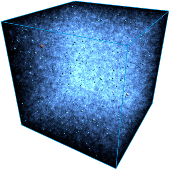
OuterRim N-body simulation:
27 mocks from the $\left(3~\mathrm{Gpc}.h^{-1}\right)^3$ box at $z=0$

Apply selection:
- Photo-detection: 2 points with SNR $>$ 5
- Spectro-typing selection from the ZTF Bright Transient Survey paper

Velocity estimator: velocities from Hubble diagram residuals
Standard candles
Standard candles + velocities
Standard candles + velocities + noise


The velocity estimator:
$$\hat{v} = -\frac{\ln(10)c}{5}\left(\frac{(1+z)c}{H(z)r(z)} - 1\right)^{-1}\Delta\mu$$
The velocity estimator:
$$\sigma_\hat{v} = -\frac{\ln(10)c}{5}\left(\frac{(1+z)c}{H(z)r(z)} - 1\right)^{-1}\sigma_\mu$$
The Maximum-Likelihood method
We can approximate the velocity field as a Gaussian random field
\(\mathbf{p}_\mathrm{HD} = \left\{M_0, \alpha, \beta, \sigma_M\right\}\) are the SNe Ia Hubble diagram parameters
\(\mathbf{p} = \left\{f\sigma_8, \sigma_v, \sigma_u\right\}\) are growth-rate related parameters
\(C_{ij}(\mathbf{p}, \mathbf{p}_\mathrm{HD}) = C_{ij}^{vv}(f\sigma_8, \sigma_u) + (\sigma_v^2 + \sigma_\hat{v}^2(\mathbf{p}_{HD}))\delta_{ij}\) the covariance matrix
$C_{ij}^{vv} \propto (f\sigma_8)^2\int_0^{+\infty}{P_{\theta\theta}(k)D_u^2(k)W_{ij}(k) dk}$
$P_{\theta\theta}\equiv$ Power spectrum of velocity divergence
$D_u = \mathrm{sinc}(\sigma_u k)\equiv$ Damping factor to account for RSD effect
$W_{ij}(k) = W(\mathbf{x}_i, \mathbf{x}_j; k)\equiv$ Window funtion

Results: The selection bias
The sample bias appears on Hubble diagram residuals at \(z \sim 0.06\) and grows up to \(\Delta\mu \sim -0.13\) at \(z \sim 0.12\)
It gives a positive bias on estimated peculiar velocities


$$\hat{v} = -\frac{\ln(10)c}{5}\left(\frac{(1+z)c}{H(z)r(z)} - 1\right)^{-1}\Delta\mu$$

That results to a bias on $f\sigma_8$

Results: ZTF 6-years complete sample
We can build a bias free sample by applying a redshift cut at \(z = 0.06\).
$\langle N_\mathrm{SN} \rangle \simeq 1620 \sim$ half of the sample
Results for our 27 mocks :
- Fit with $v_\mathrm{true}$: $\frac{\langle f\sigma_8 \rangle }{(f\sigma_8)_\mathrm{fid}} = 0.991 \pm 0.016 $, $\frac{\sqrt{\left<\sigma_{f \sigma_8}^2\right>}}{(f\sigma_8)_\mathrm{fid}} = 0.100$
- Fit fixing $\mathbf{p}_\mathrm{HD}$: $\frac{\langle f\sigma_8 \rangle }{(f\sigma_8)_\mathrm{fid}} = 1.036 \pm 0.031$, $\frac{\sqrt{\left<\sigma_{f \sigma_8}^2\right>}}{(f\sigma_8)_\mathrm{fid}} = 0.185$
- Fit with $\mathbf{p}$, $\mathbf{p}_\mathrm{HD}$ free: $\frac{\langle f\sigma_8 \rangle }{(f\sigma_8)_\mathrm{fid}} = 0.998 \pm 0.037$, $\frac{\sqrt{\left<\sigma_{f \sigma_8}^2\right>}}{(f\sigma_8)_\mathrm{fid}} = 0.188$
Comparaison with existing measurements

With only ~1600 SNe ZTF is at the same precision level than existing measurements with several thousands of galaxies !
How to improve the measurement?
Debias the velocity estimates ?
How to improve the measurement? Debias velocities
Simulate a perfect correction of the bias:
$v_{\mathrm{debias}, i} \sim \mathcal{N}(v_\mathrm{true}, \sigma_{\hat{v}, i})$


The error on $f\sigma_8$ reduce from $17 \%$ to $15 \%$
Density drops rapidly after $z=0.06$ and errors on $\hat{v}_p$ increase ~linearly with $z$
How to improve the measurement?
-
Debias the velocity estimates ?
Does not improve much the constraint on $f\sigma_8$
-
Use photo-typing to increase the redshift limit
DESC project presented by Damiano Rosselli
-
Combinaison with RSD measurements (e.g. ZTF + DESI)
Ongoing work on this at CPPM by Julian Bautista
Conclusion
We developed and run a full detailed simulation and analysis pipeline to measure growth rate of structure using ZTF SNe Ia
Our analysis shows that the spectroscopic selection causes a bias for $f\sigma_8$ when using SNe Ia at $z>0.06$
We forecast that a 6-years ZTF SNe Ia spectro-identified sample cut at $z=0.06$ will produce a $f\sigma_8$ measurement with a precision of $\sim 19\%$ using velocities only
Correcting the bias does not improve much the constraint on $f\sigma_8$ but significant improvements are expected from future work on photometric typing analysis and combination with RSD
Thanks for your attention !!!
Backup slides
BTS selection function

$f\sigma_8$ in function of $z_\mathrm{max}$


Velocity estimators bias
$\hat{v}_2 = -\frac{\ln(10)}{5}\frac{H(z)r(z)}{(1+z)}\Delta\mu$
$\hat{v}_4 = -\frac{\ln(10)c}{5}\frac{z}{1+z}\Delta\mu$

Gaussian prior on $\sigma_u$


