Growth-rate measurement with type Ia supernovae
Bastien Carreres,
J. E. Bautista, F. Feinstein, D. Fouchez, B. Racine, M. Smith et al.
Image credits: ZTF.Caltech
Why measuring the growth rate of cosmic structures?
We live in an universe in accelerated expansion!
Could it be due to a dark energy constant?
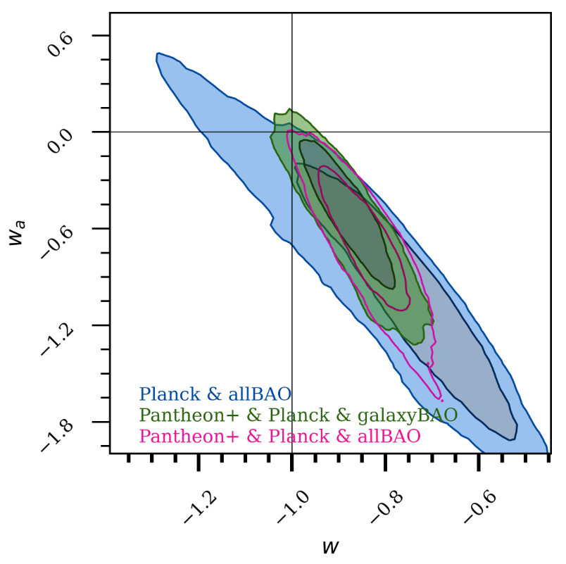
Could it be due to a dynamical dark energy field?
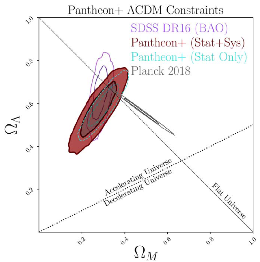
Credits: Pantheon+ Analysis Brout et al. 2022
Why measuring the growth rate of cosmic structures?
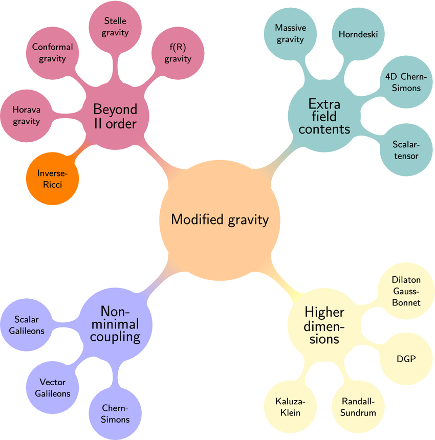
Alternative: GR is not valid at all scales and we need modified gravity models

Image credits: DALL.E
Luckily:
Those models have expansion history hard to distinguish from $\Lambda$CDM...
...but they affect structures formation !
Image credits: arXiv:2204.06533
\(f\sigma_8\) as a probe for general relativity
Structure evolution: Dark energy vs Gravity
Density contrast in linear theory:
$\delta(a, \mathbf{x}) = D(a)\tilde{\delta}(\mathbf{x})$
where $D(a) \equiv$ growth factor
In measurement we use: $\sigma_8 \propto D$
Velocities are linked to density through continuity equation:
$\nabla.v = -aH\frac{d\delta}{da}\ \propto -aHf\sigma_8\delta$
where $f = \frac{d \ln D}{d\ln a} \equiv$ growth rate
In $\Lambda$CDM + GR:
$f \simeq \Omega_m^\gamma$ with $\gamma \simeq 0.55$

Image credits: Illustris TNG
How to measure $f\sigma_8$ ?
Velocities as probes of $f\sigma_8$:
$\nabla.v \propto f\sigma_8$
Doppler effect on redshift:
$1 + z_\mathrm{obs} = \left(1 + z_\mathrm{cos}\right)\left(1 + \frac{v_p}{c}\right)$
Indirect method: Redshift Space Distorsions of the density field
Velocities leads to distorted positions: $r(z_\mathrm{obs}) \simeq r(z_\mathrm{cos})+ \frac{1+z_\mathrm{cos}}{H(z_\mathrm{cos})}v_p$
Direct method: velocity tracers
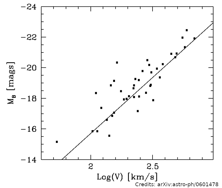
Galaxies Tully-Fisher and Fundamental Plane: $\sigma_D/D \sim 20\%$
Type Ia supernovae: $\sigma_D/D \sim 7 \%$
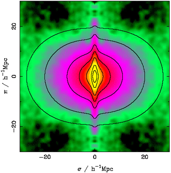
Linear RSD

Non-linear RSD

2D corr. from Peacock et al. 2001


Tully-Fisher relation
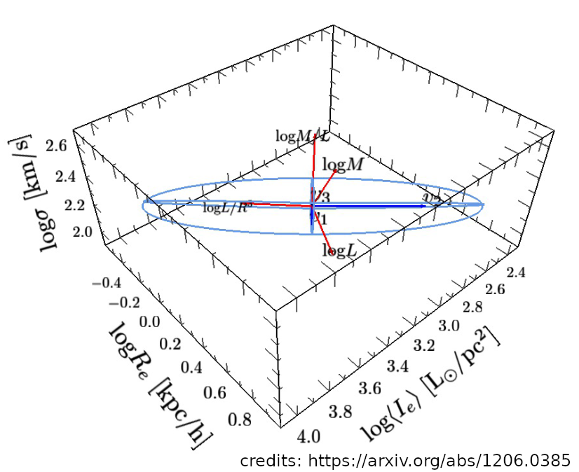
Fundamental-Plane relation
RSD
Velocity tracers
New player in the game: large low-z SNe Ia sample from the Zwicky Transient Facility !
Image credits: Illustris TNG
The Zwicky Transient Facility survey
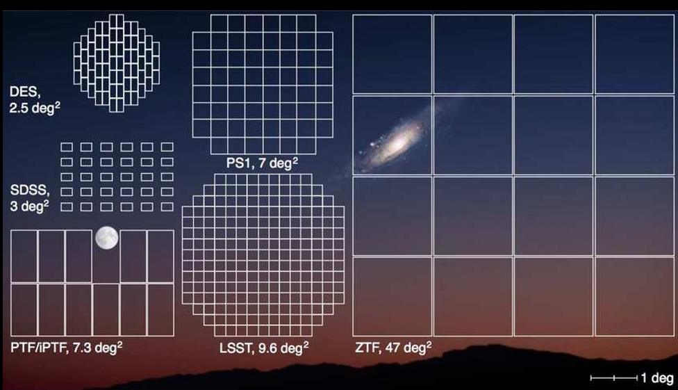
The ZTF camera at Palomar observatory observes the full North hemisphere each night in 2 (g and r bands) + 1 (i band)
Already $\sim 8000$ classified supernovae
$\sim 5000$ SNe Ia at low redshift $z < 0.1$

Image credits: ZTF.Caltech
The Zwicky Transient Facility survey: spectroscopic follow-up
The Bright Transient Survey types every ZTF transients with $mag < 17$
Typing efficiency is magnitude limited
No typing for $mag > 19$

Image credits: ZTF.Caltech
The simulation and analysis pipeline
Use of ZTF existing observations as input for the simulation.
Includes observing strategy, filters, sky noise...
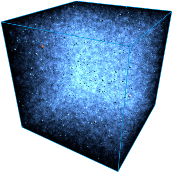
OuterRim N-body simulation:
We create 27 mocks of $\left(1~\mathrm{Gpc}.h^{-1}\right)^3 \ \left(z_\mathrm{max} \simeq 0.17\right)$
from the $\left(3~\mathrm{Gpc}.h^{-1}\right)^3$ box at $z=0$

Apply selection:
- Photo-detection: 2 points with SNR $>$ 5
- Spectro-typing selection from the ZTF Bright Transient Survey paper

Velocity estimator: velocities from Hubble diagram residuals
Standard candles
Standard candles + velocities
Standard candles + velocities + noise


The velocity estimator:
$$\hat{v} = -\frac{\ln(10)c}{5}\left(\frac{(1+z)c}{H(z)r(z)} - 1\right)^{-1}\Delta\mu$$
The velocity estimator error:
$$\sigma_\hat{v} = -\frac{\ln(10)c}{5}\left(\frac{(1+z)c}{H(z)r(z)} - 1\right)^{-1}\sigma_\mu$$
The Maximum-Likelihood method (Johnson et al. 2014)
We can approximate the velocity field as a Gaussian random field
The correlation function depends of the Power Spectrum:
For densities:
$\langle\delta(\mathbf{x}_i)\delta(\mathbf{x}_i + \mathbf{r})\rangle \propto \int dk k^2 P(k) W^{(\delta)}(k;\mathbf{r}) \propto
\sigma_8^2 \int dk k^2 \tilde{P}(k)W^{(\delta)}(k; \mathbf{r})$
For velocities:
$\langle v(\mathbf{x}_i)v(\mathbf{x}_j)\rangle \propto (f\sigma_8)^2 \int dk \tilde{P}(k) W^{(v)}(k; \mathbf{x}_i, \mathbf{x}_j)$
It gives us a $f\sigma_8$ dependant model for our covariance matrix!
$C_{ij}^{vv}(f\sigma_8) = \langle v(\mathbf{x}_i)v(\mathbf{x}_j)\rangle$
Free parameters of the likelihood:
${\color{orange} \mathbf{p}_{HD} = \left\{\alpha, \beta, M_B, \sigma_M \right\}}$
${\color{yellow} \mathbf{p} = \left\{f\sigma_8, \sigma_u, \sigma_v \right\}}$, $\sigma_u \equiv$ RSD, $\sigma_v\equiv$ non-linearities
The likelihood:
$\mathcal{L}({\color{yellow}\mathbf{p}}, {\color{orange}\mathbf{p}_{\rm HD}}) \propto |C({\color{yellow}\mathbf{p}}, {\color{orange}\mathbf{p}_{\rm HD}})|^{-\frac{1}{2}} \times\exp\left[-\frac{1}{2}\mathbf{v}^T({\color{orange}\mathbf{p}_{\rm HD}})C({\color{yellow}\mathbf{p}}, {\color{orange}\mathbf{p}_{\rm HD}})^{-1}\mathbf{v}({\color{orange}\mathbf{p}_{\rm HD}})\right]$$C^{vv}_{ij}({\color{yellow}f\sigma_8}, {\color{yellow}\sigma_u}) = \langle v(\mathbf{x}_i)v(\mathbf{x}_j)\rangle \propto ({\color{yellow}f\sigma_8})^2 \int dk P(k) W(k) D(k; {\color{yellow}\sigma_u}) $

Results: the selection bias
Magnitude limited selection $\Rightarrow$ Selection bias: when redshift increases, only brighter objects are detected
Bias on HD residuals

Bias on velocity estimates

$$\hat{v} = -\frac{\ln(10)c}{5}\left(\frac{(1+z)c}{H(z)r(z)} - 1\right)^{-1}\Delta\mu$$

Only the estimated velocities are biased !!!
Bias on $f\sigma_8$

Results: forecast for a ZTF 6-years complete sample
We can build a bias free sample by applying a redshift cut at \(z = 0.06\).
$\langle N_\mathrm{SN} \rangle \simeq 1620 \sim$ half of the sample
Results for our 27 mocks :
- Fit with $v_\mathrm{true}$: $\frac{\langle f\sigma_8 \rangle }{(f\sigma_8)_\mathrm{fid}} = 0.991 \pm 0.016 $, $\frac{\sqrt{\left<\sigma_{f \sigma_8}^2\right>}}{(f\sigma_8)_\mathrm{fid}} = 0.100$
- Fit fixing $\mathbf{p}_\mathrm{HD}$: $\frac{\langle f\sigma_8 \rangle }{(f\sigma_8)_\mathrm{fid}} = 1.036 \pm 0.031$, $\frac{\sqrt{\left<\sigma_{f \sigma_8}^2\right>}}{(f\sigma_8)_\mathrm{fid}} = 0.185$
- Fit with $\mathbf{p}$, $\mathbf{p}_\mathrm{HD}$ free: $\frac{\langle f\sigma_8 \rangle }{(f\sigma_8)_\mathrm{fid}} = 0.998 \pm 0.037$, $\frac{\sqrt{\left<\sigma_{f \sigma_8}^2\right>}}{(f\sigma_8)_\mathrm{fid}} = 0.188$
Comparison with existing measurements

With only ~1600 SNe Ia, ZTF is at the same precision level than existing measurements with several thousands of galaxies !
How to improve the measurement?
Bias correction of the velocity estimates ?
How to improve the measurement? Bias correction of the velocities
Simulate a perfect correction of the bias:
$v_{\mathrm{debias}, i} \sim \mathcal{N}(v_\mathrm{true}, \sigma_{\hat{v}, i})$


From a redshift limit of $z \sim 0.06$ to $z\sim 0.13$, $N_{SN}$ is doubled but the error on $f\sigma_8$ only reduces from $17
\%$ to $15 \%$
Sampling drops rapidly after $z=0.06$ and errors on $\hat{v}_p$ increase ~linearly with $z$
How to improve the measurement?
-
Bias correction of the velocity estimates ?
Does not improve the constraint on $f\sigma_8$
-
Use photo-typing to increase the redshift limit
DESC project led by Damiano Rosselli
-
Combination with RSD measurements (e.g. ZTF + DESI)
Ongoing work on this at CPPM by Julian Bautista
Future surveys

Peculiar velocities + RSD will put strong constraint on $f\sigma_8$ at low redshift
Forecast credits: DESI arxiv:1611.00036, LSST arxiv:1708.08236, EUCLID arXiv:1606.00180
Conclusion
We developed and ran a full detailed simulation and analysis pipeline to measure the growth rate of structure using ZTF SNe Ia
The spectroscopic selection causes a bias for $f\sigma_8$ above $z\sim0.06$
We forecast that a 6-year ZTF SNe Ia spectro-identified sample cut at $z=0.06$ will produce a $f\sigma_8$ measurement with a precision of $\sim 19\%$
Significant improvements are expected from future work on photometric typing analysis and combination with RSD
Thanks for your attention !!!
Backup slides
$f\sigma_8$ as a function of $z_\mathrm{max}$


Velocity estimators biases
$\hat{v}_2 = -\frac{\ln(10)}{5}\frac{H(z)r(z)}{(1+z)}\Delta\mu$
$\hat{v}_4 = -\frac{\ln(10)c}{5}\frac{z}{1+z}\Delta\mu$

Gaussian prior on $\sigma_u$

